Overview
This article is a visual gallery for clover’s modification heatmap
functions. It covers every parameter of plot_mod_heatmap()
and prep_mod_heatmap(), plus the related
plot_bcerror_profile() and
plot_mod_landscape() functions.
All examples use the bundled E. coli base-calling error data shipped with the package.
Data preparation
The bundled RDS contains pre-summarized bcerror data comparing
wild-type (wt) and TruB-deletion (tb) E.
coli across 10 tRNAs.
bcerror_rds <- readRDS(clover_example("ecoli/bcerror_summary.rds"))
bcerror_summary <- bcerror_rds$bcerror_summary
bcerror_charged <- bcerror_rds$bcerror_charged
Compute the per-position delta (wt minus TruB-del). Positive values mean higher error in wild-type, indicating a modification lost in the mutant.
bcerror_delta <- compute_bcerror_delta(bcerror_summary, delta = wt - tb)
bcerror_delta
#> # A tibble: 796 × 5
#>    ref                     pos     tb     wt     delta
#>    <chr>                 <int>  <dbl>  <dbl>     <dbl>
#>  1 host-tRNA-Asn-GTT-1-1     1 0.0334 0.0405  0.00711
#>  2 host-tRNA-Asn-GTT-1-1     2 0.0660 0.0896  0.0236
#>  3 host-tRNA-Asn-GTT-1-1     3 0.0587 0.0809  0.0221
#>  4 host-tRNA-Asn-GTT-1-1     4 0.195  0.201   0.00584
#>  5 host-tRNA-Asn-GTT-1-1     5 0.258  0.288   0.0292
#>  6 host-tRNA-Asn-GTT-1-1     6 0.117  0.134   0.0170
#>  7 host-tRNA-Asn-GTT-1-1     7 0.125  0.133   0.00720
#>  8 host-tRNA-Asn-GTT-1-1     8 0.0644 0.0706  0.00617
#>  9 host-tRNA-Asn-GTT-1-1     9 0.0623 0.0619 -0.000387
#> 10 host-tRNA-Asn-GTT-1-1    10 0.0295 0.0266 -0.00295
#> # ℹ 786 more rows
Preparing heatmap data
prep_mod_heatmap() joins Sprinzl coordinates, optionally
annotates known modifications from MODOMICS, and shortens tRNA names for
display.
sprinzl <- read_sprinzl_coords(
  clover_example("sprinzl/ecoliK12_global_coords.tsv.gz")
)
trna_fasta <- clover_example("ecoli/trna_only.fa.gz")
mods <- modomics_mods(trna_fasta, organism = "Escherichia coli")

heatmap_data <- prep_mod_heatmap(
  bcerror_delta,
  sprinzl_coords = sprinzl,
  mods = mods
)

heatmap_data
#> # A tibble: 795 × 10
#>    ref     pos     tb     wt    delta trna_id sprinzl_label global_index has_mod
#>    <chr> <dbl>  <dbl>  <dbl>    <dbl> <chr>   <fct>                <dbl> <lgl>
#>  1 tRNA…     1 0.0334 0.0405  7.11e-3 tRNA-A… 1                        1 FALSE
#>  2 tRNA…     2 0.0660 0.0896  2.36e-2 tRNA-A… 2                        2 FALSE
#>  3 tRNA…     3 0.0587 0.0809  2.21e-2 tRNA-A… 3                        3 FALSE
#>  4 tRNA…     4 0.195  0.201   5.84e-3 tRNA-A… 4                        4 FALSE
#>  5 tRNA…     5 0.258  0.288   2.92e-2 tRNA-A… 5                        5 FALSE
#>  6 tRNA…     6 0.117  0.134   1.70e-2 tRNA-A… 6                        6 FALSE
#>  7 tRNA…     7 0.125  0.133   7.20e-3 tRNA-A… 7                        7 FALSE
#>  8 tRNA…     8 0.0644 0.0706  6.17e-3 tRNA-A… 8                        8 TRUE
#>  9 tRNA…     9 0.0623 0.0619 -3.87e-4 tRNA-A… 9                        9 FALSE
#> 10 tRNA…    10 0.0295 0.0266 -2.95e-3 tRNA-A… 10                      10 FALSE
#> # ℹ 785 more rows
#> # ℹ 1 more variable: trna_label <chr>
The result is a tibble with sprinzl_label as an ordered
factor (canonical tRNA position ordering), trna_label for
compact y-axis names, and has_mod marking known MODOMICS
modification sites.
Basic heatmap
The simplest call passes the prepared data with appropriate column mappings.
plot_mod_heatmap(
  heatmap_data,
  value_col = "delta",
  ref_col = "trna_label"
)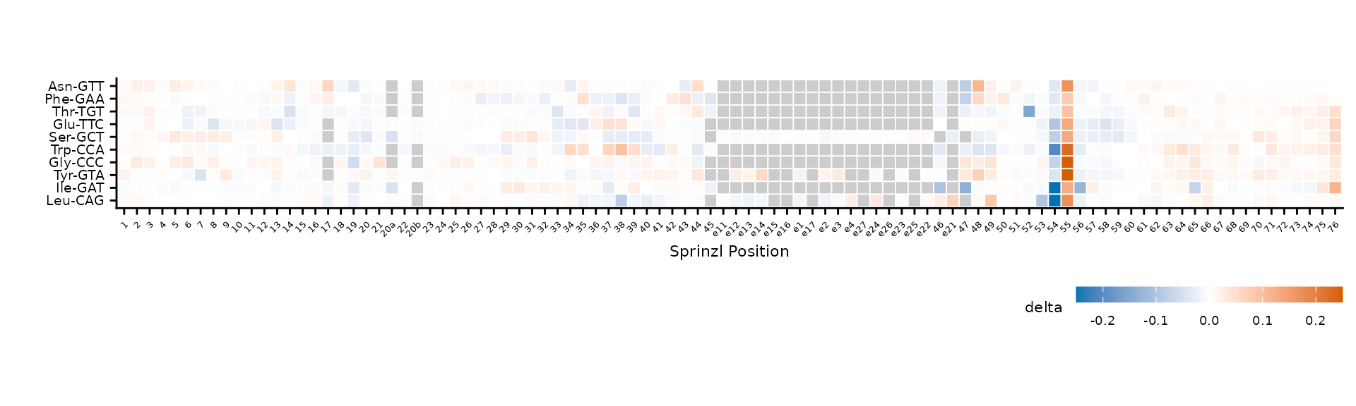
Basic modification heatmap with default settings.
Color scale
Control the diverging color scale with color_limits,
color_low, color_high, and
na_value.
plot_mod_heatmap(
  heatmap_data,
  value_col = "delta",
  ref_col = "trna_label",
  color_limits = c(-0.1, 0.1),
  color_low = "#7B3294",
  color_high = "#008837",
  na_value = "gray95"
)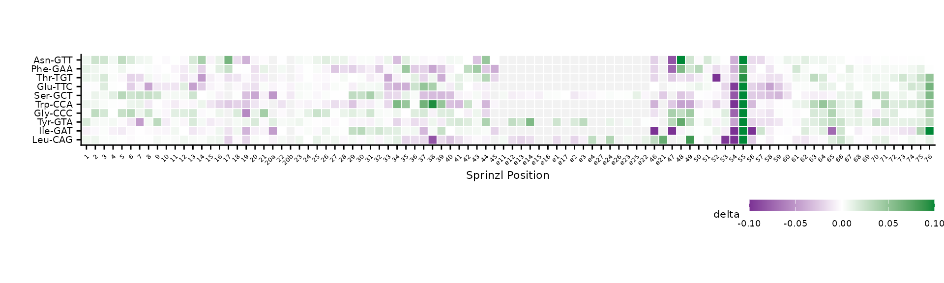
Custom color scale with tighter limits and purple-green palette.
The default palette uses colorblind-friendly blue
(#0072B2) and vermillion (#D55E00). Values
outside color_limits are squished to the extremes.
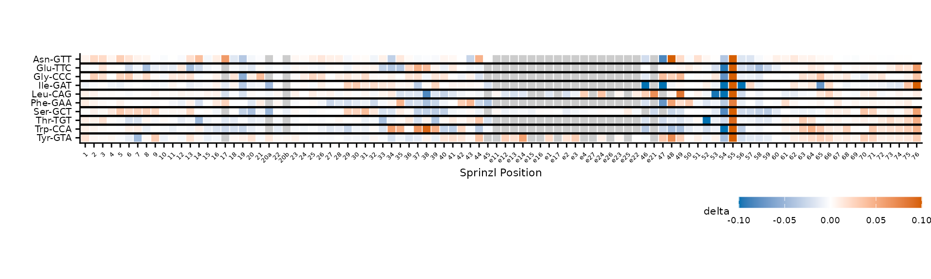
Clustering
By default, rows are clustered using Ward’s D2 hierarchical
clustering on the Sprinzl-position value matrix. Set
cluster = FALSE to keep alphabetical order.
plot_mod_heatmap(
  heatmap_data,
  value_col = "delta",
  ref_col = "trna_label",
  color_limits = c(-0.1, 0.1)
)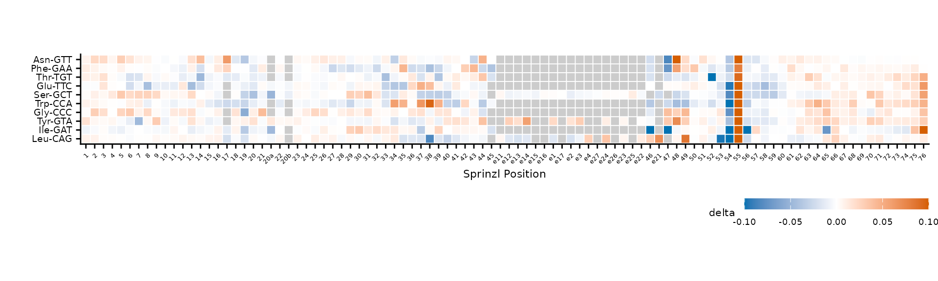
Clustered rows (default).
plot_mod_heatmap(
  heatmap_data,
  value_col = "delta",
  ref_col = "trna_label",
  cluster = FALSE,
  color_limits = c(-0.1, 0.1)
)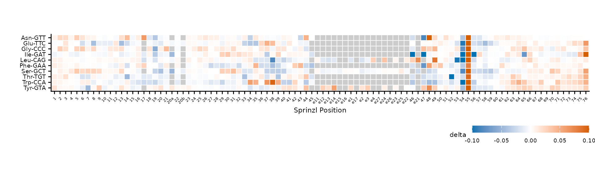
Alphabetical row order (cluster = FALSE).
Noise filtering with cluster_threshold
When clustering, low-level noise can dominate the distance matrix.
Setting cluster_threshold restricts clustering to positions
where at least one tRNA exceeds the threshold in absolute value.
plot_mod_heatmap(
  heatmap_data,
  value_col = "delta",
  ref_col = "trna_label",
  color_limits = c(-0.1, 0.1),
  cluster_threshold = 0.05
)
Clustering uses only positions with |delta| > 0.05.
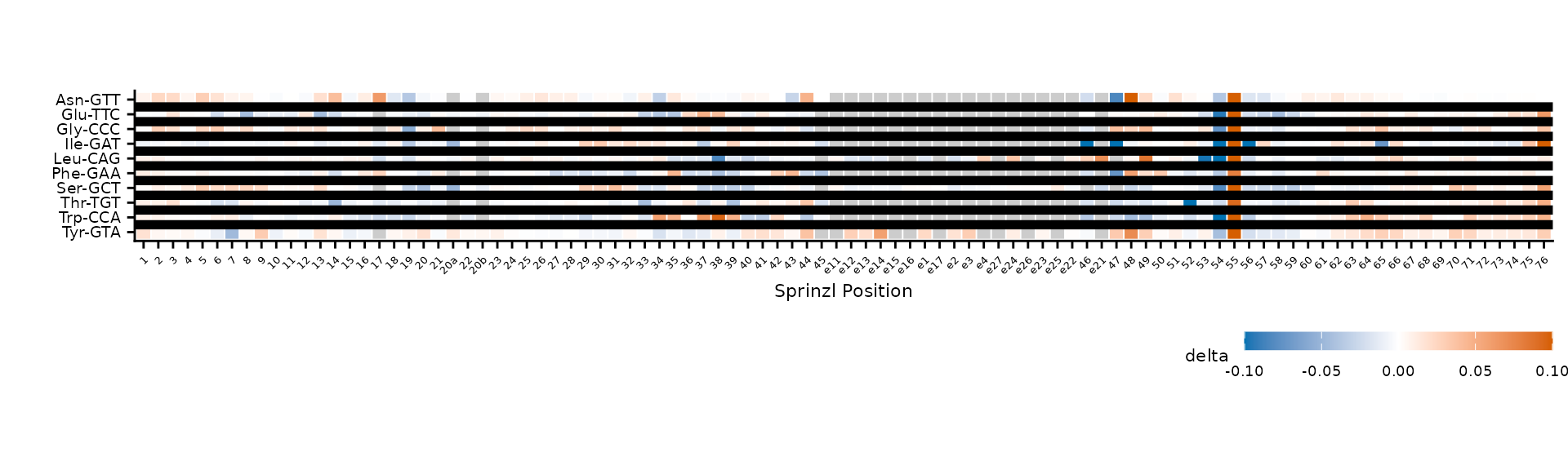
Group-aware clustering
When tRNAs belong to natural groups (e.g., amino acid families), use
group_col to cluster within each group and draw horizontal
dividers between them. First, add an amino acid column to the data.
plot_mod_heatmap(
  heatmap_grouped,
  value_col = "delta",
  ref_col = "trna_label",
  color_limits = c(-0.1, 0.1),
  group_col = "amino_acid"
)
Clustering within amino acid groups, separated by dividers.
Control the divider line thickness with
divider_linewidth.
plot_mod_heatmap(
  heatmap_grouped,
  value_col = "delta",
  ref_col = "trna_label",
  color_limits = c(-0.1, 0.1),
  group_col = "amino_acid",
  divider_linewidth = 2
)
Thicker dividers between groups.
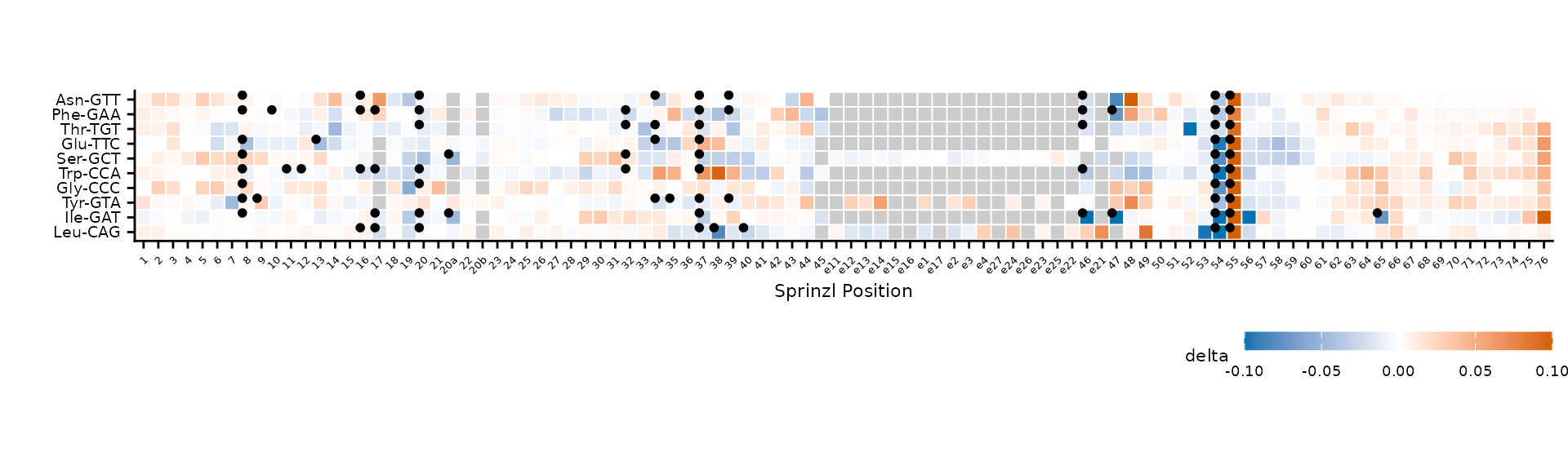
Modification highlights
When prep_mod_heatmap() is called with
mods, a logical has_mod column marks known
modification sites. Use highlight_col to overlay dots on
those cells.
plot_mod_heatmap(
  heatmap_data,
  value_col = "delta",
  ref_col = "trna_label",
  color_limits = c(-0.1, 0.1),
  highlight_col = "has_mod"
)
MODOMICS modification sites marked with dots.
Adjust dot appearance with highlight_size and
highlight_offset (x/y displacement from tile center).
plot_mod_heatmap(
  heatmap_data,
  value_col = "delta",
  ref_col = "trna_label",
  color_limits = c(-0.1, 0.1),
  highlight_col = "has_mod",
  highlight_size = 1.2,
  highlight_offset = c(-0.3, 0.3)
)
Larger highlight dots with custom offset.
Tile labels
Overlay text on tiles with label_col. Labels are only
shown where abs(value) >= label_min, and text color
automatically switches between black and white for contrast.
# Add the reference base at each position for labeling
ref_seqs <- Biostrings::readDNAStringSet(trna_fasta)
ref_bases <- tibble::tibble(
  ref = sub("^host-", "", rep(names(ref_seqs), Biostrings::width(ref_seqs))),
  pos = unlist(lapply(Biostrings::width(ref_seqs), seq_len)),
  ref_base = strsplit(as.character(unlist(ref_seqs)), "") |> unlist()
)

heatmap_labeled <- heatmap_data |>
  left_join(ref_bases, by = c("ref", "pos"))
plot_mod_heatmap(
  heatmap_labeled,
  value_col = "delta",
  ref_col = "trna_label",
  color_limits = c(-0.1, 0.1),
  label_col = "ref_base",
  label_min = 0.03,
  label_size = 2
)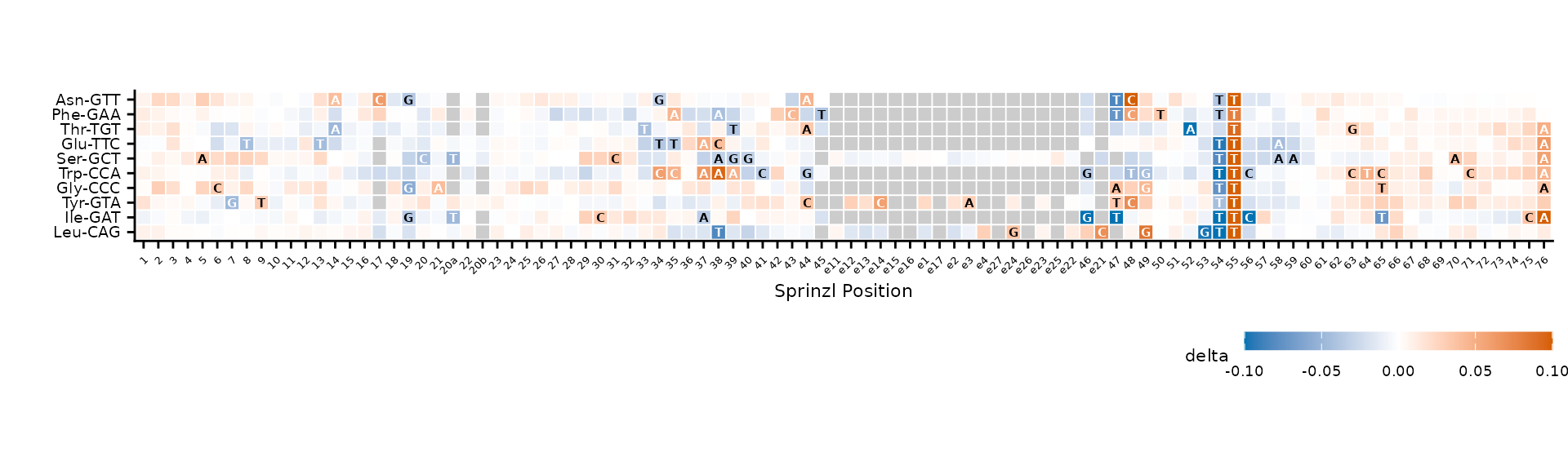
Reference bases overlaid on tiles where |delta| >= 0.03.
Legend and caption
Customize the fill legend with fill_name and
fill_breaks, and add explanatory text with
caption.
plot_mod_heatmap(
  heatmap_data,
  value_col = "delta",
  ref_col = "trna_label",
  color_limits = c(-0.1, 0.1),
  fill_name = "\u0394 error rate",
  fill_breaks = c(-0.1, -0.05, 0, 0.05, 0.1),
  caption = "Positive values = higher error in wt (modification present in wt, lost in TruB-del)."
)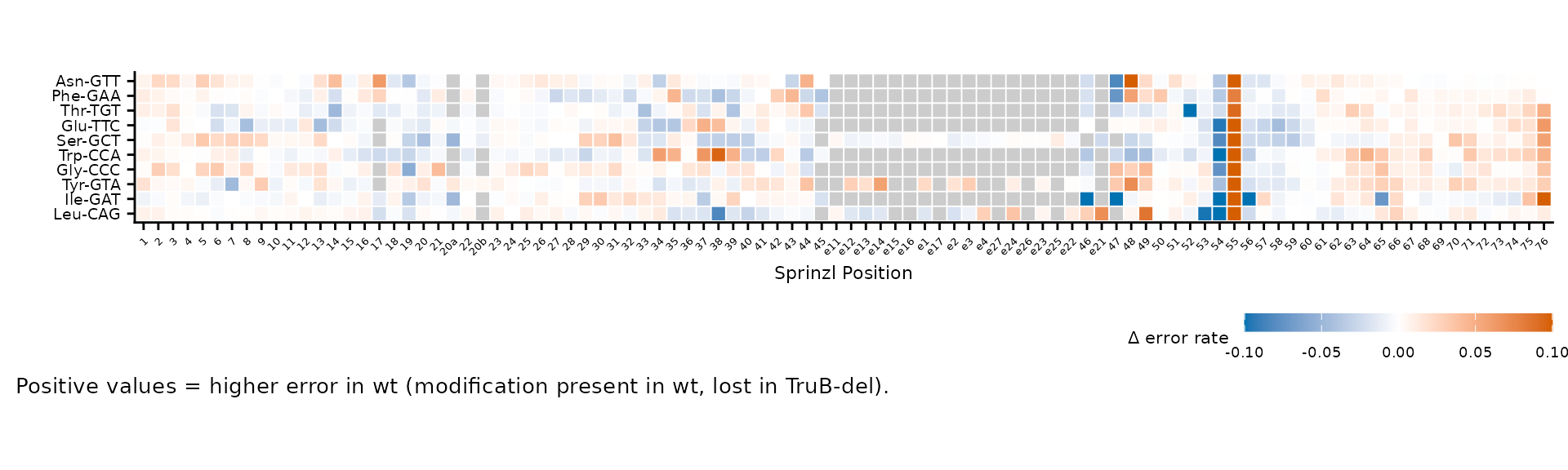
Custom legend title, breaks, and caption.
Square versus free aspect ratio
By default, square = TRUE uses
coord_fixed(ratio = 1) for square tiles. Set
square = FALSE to let ggplot2 fill the available space,
which is useful for wide heatmaps with many positions.
plot_mod_heatmap(
  heatmap_data,
  value_col = "delta",
  ref_col = "trna_label",
  color_limits = c(-0.1, 0.1),
  square = FALSE
)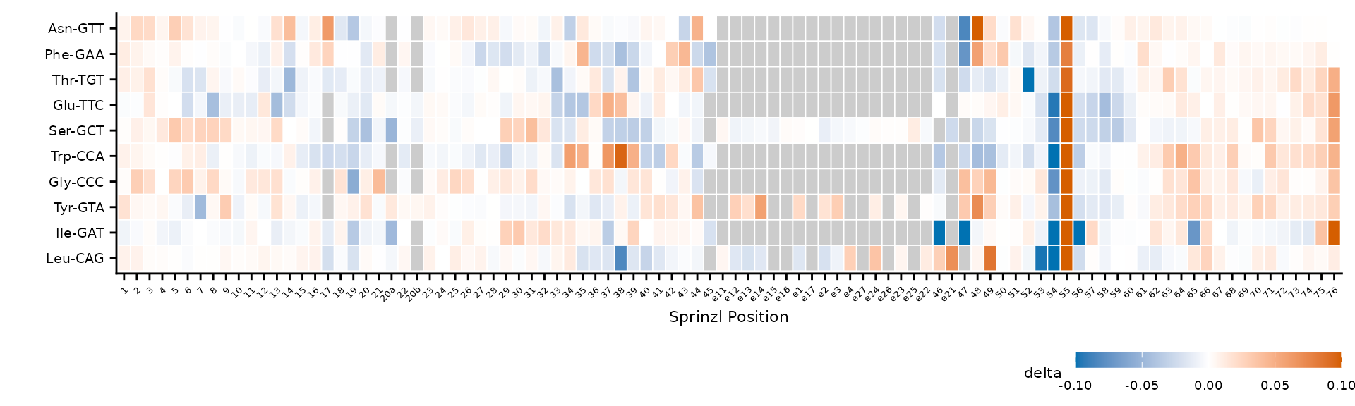
Free aspect ratio stretches tiles to fill the plot area.
Base-calling error profiles
plot_bcerror_profile() creates line plots of
per-position error rates, faceted by tRNA and colored by condition.
plot_trnas <- c(
  "host-tRNA-Asn-GTT-1-1",
  "host-tRNA-Glu-TTC-1-1",
  "host-tRNA-Phe-GAA-1-1"
)

plot_bcerror_profile(bcerror_summary, refs = plot_trnas)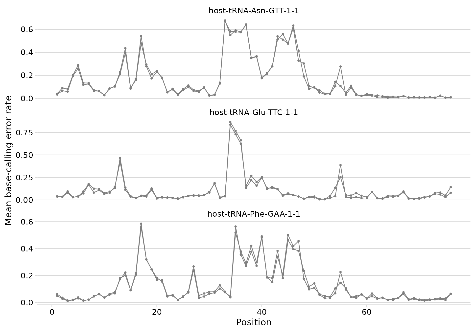
Error profiles for three tRNAs.
Adding modification annotations
Pass a mods tibble to overlay vertical dashed lines at
known modification positions.
plot_bcerror_profile(bcerror_summary, refs = plot_trnas, mods = mods)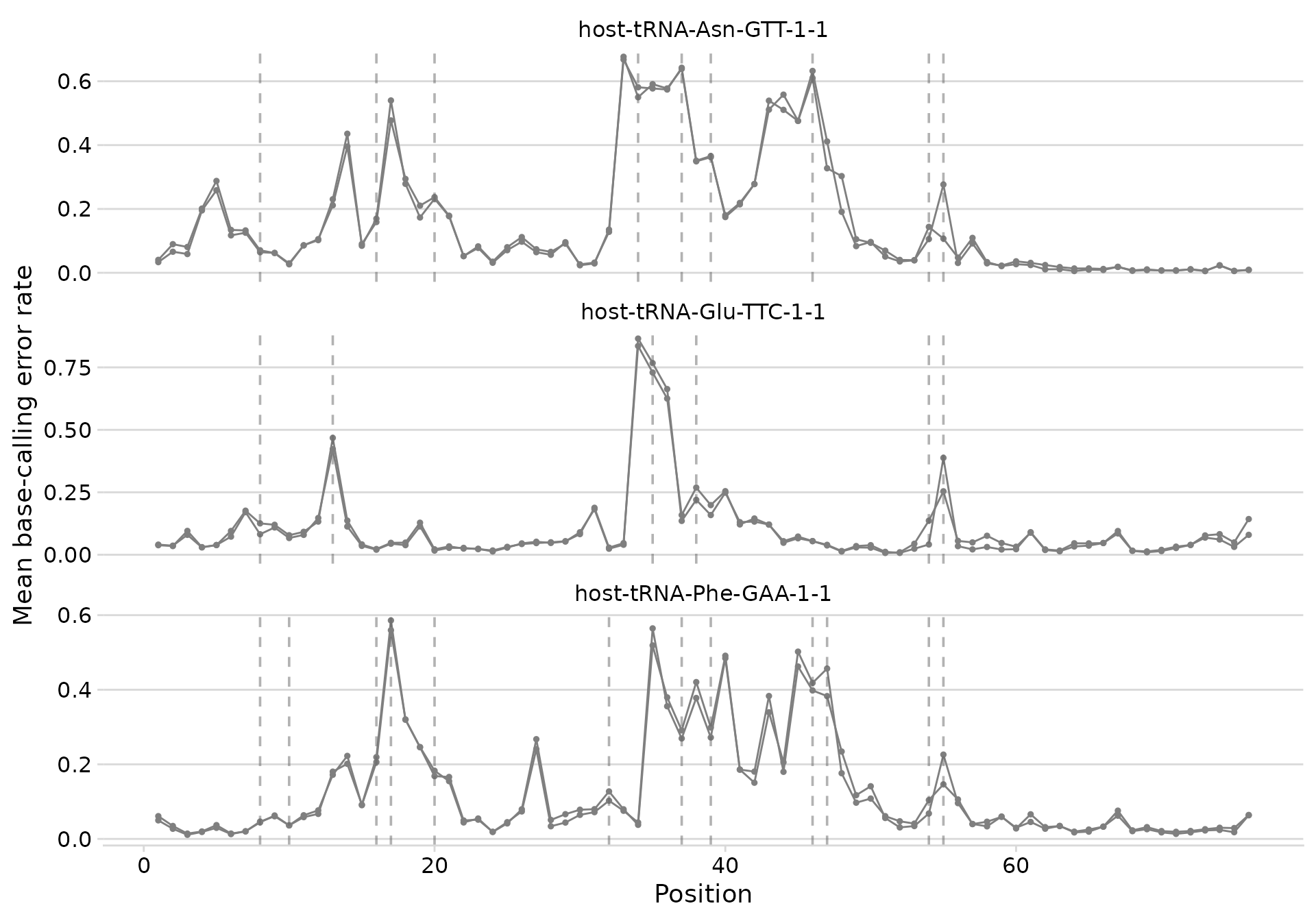
Error profiles with MODOMICS modification positions marked.
Custom colors and layout
Override condition colors with a named vector, and change the facet
layout with ncol.
plot_bcerror_profile(
  bcerror_summary,
  refs = plot_trnas,
  mods = mods,
  colors = c(wt = "#E69F00", tb = "#56B4E9"),
  ncol = 2
)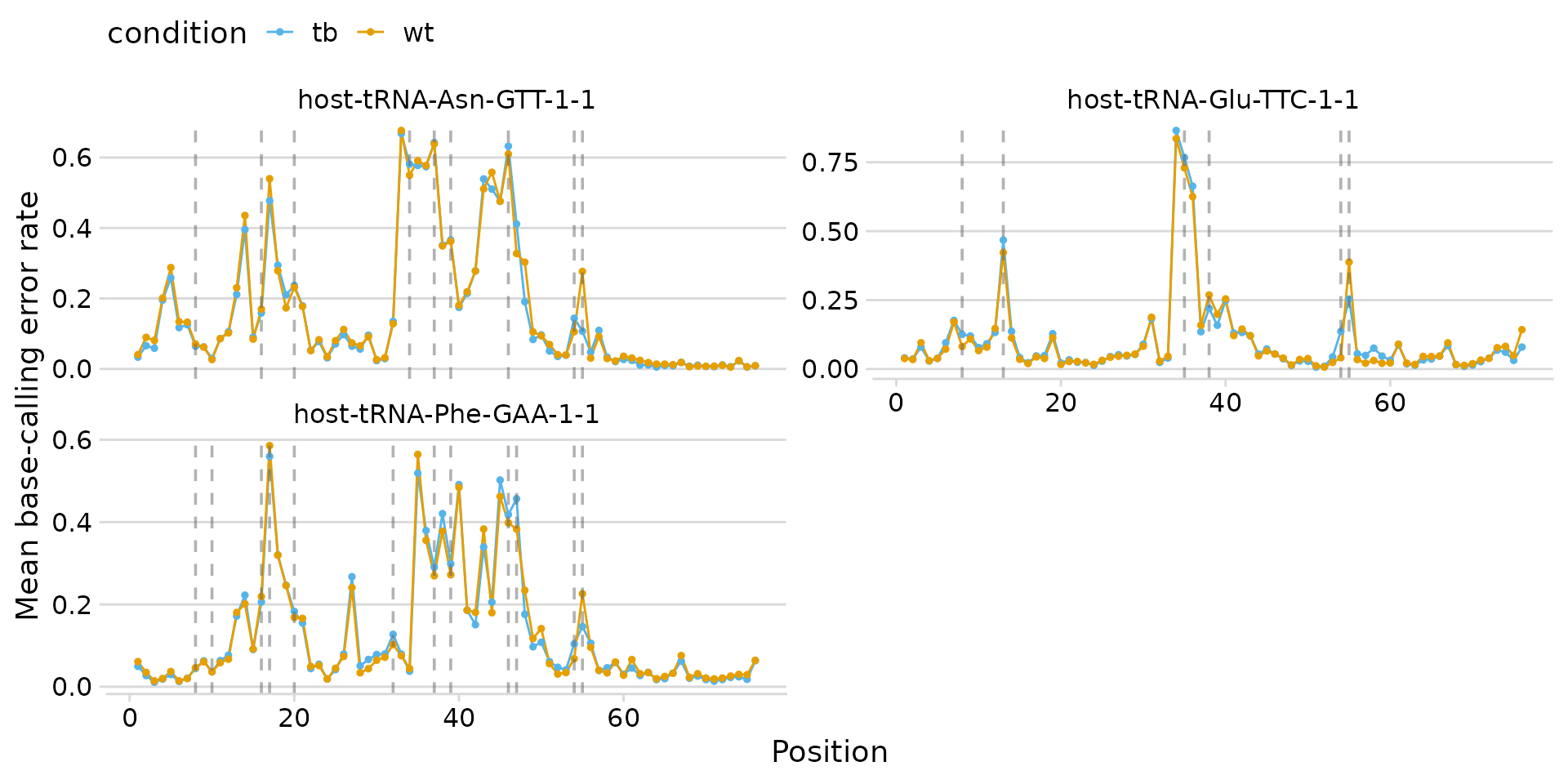
Custom colors and two-column layout.
Modification landscape
plot_mod_landscape() creates a stacked panel plot
showing multiple metrics along the tRNA sequence. Each metric gets its
own panel sharing a common x-axis. This is useful for comparing error
rates, mismatch types, or other per-position statistics side by
side.
First, prepare single-tRNA data with Sprinzl coordinates and region annotations.
# Pick one tRNA and reshape for landscape plotting
landscape_data <- bcerror_summary |>
  filter(ref == "host-tRNA-Glu-TTC-1-1", condition == "wt")

# Add Sprinzl coordinates and region info
sprinzl_glu <- sprinzl |>
  filter(trna_id == "tRNA-Glu-UUC-1-1") |>
  select(pos, sprinzl_label, region)

landscape_data <- landscape_data |>
  left_join(sprinzl_glu, by = "pos") |>
  filter(!is.na(sprinzl_label))

# Add a logical column for known modification positions
mod_positions <- mods |>
  filter(ref == "host-tRNA-Glu-TTC-1-1") |>
  distinct(pos) |>
  mutate(has_mod = TRUE)

landscape_data <- landscape_data |>
  left_join(mod_positions, by = "pos") |>
  mutate(has_mod = tidyr::replace_na(has_mod, FALSE))
plot_mod_landscape(
  landscape_data,
  metrics = c("mean_error", "mean_mis")
)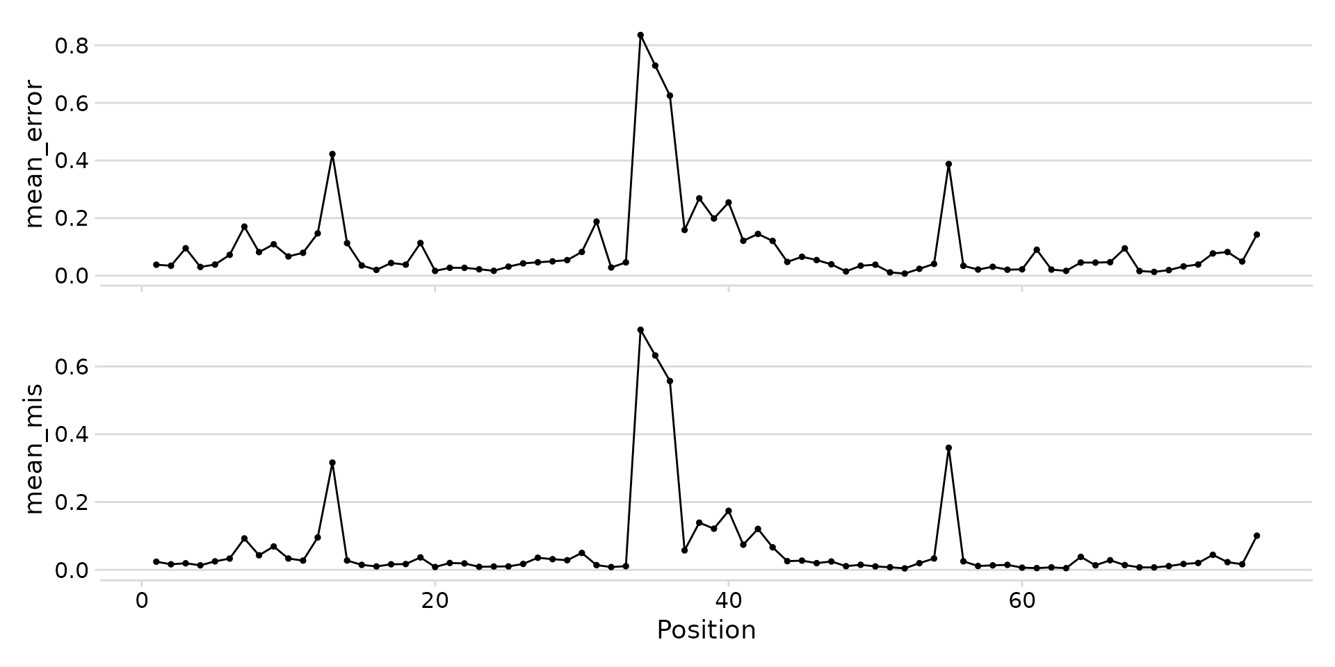
Stacked landscape of error rate and mismatch frequency.
Region shading
Pass region_col to add background shading for structural
regions (acceptor-stem, D-loop, anticodon-stem, etc.).
plot_mod_landscape(
  landscape_data,
  metrics = c("mean_error", "mean_mis"),
  region_col = "region"
)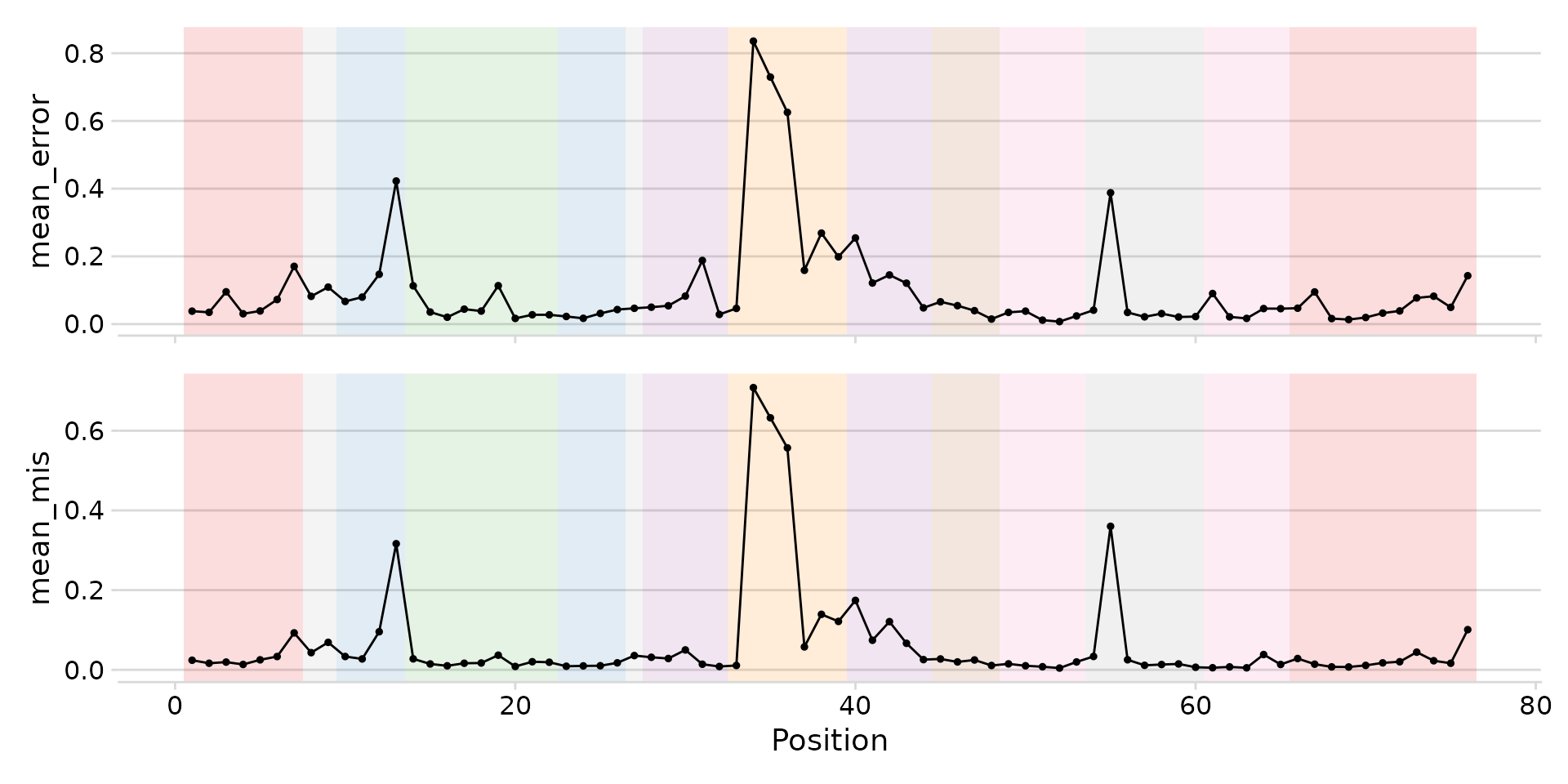
Landscape with structural region shading.
Sprinzl axis and modification highlights
Add a secondary x-axis with Sprinzl position labels using
sprinzl_col. Use mod_col to highlight known
modification positions on that axis (shown in bold orange when ggtext is
installed).
plot_mod_landscape(
  landscape_data,
  metrics = c("mean_error", "mean_mis"),
  region_col = "region",
  sprinzl_col = "sprinzl_label",
  mod_col = "has_mod",
  title = "tRNA-Glu-UUC-1-1 modification landscape",
  heights = c(2, 1)
)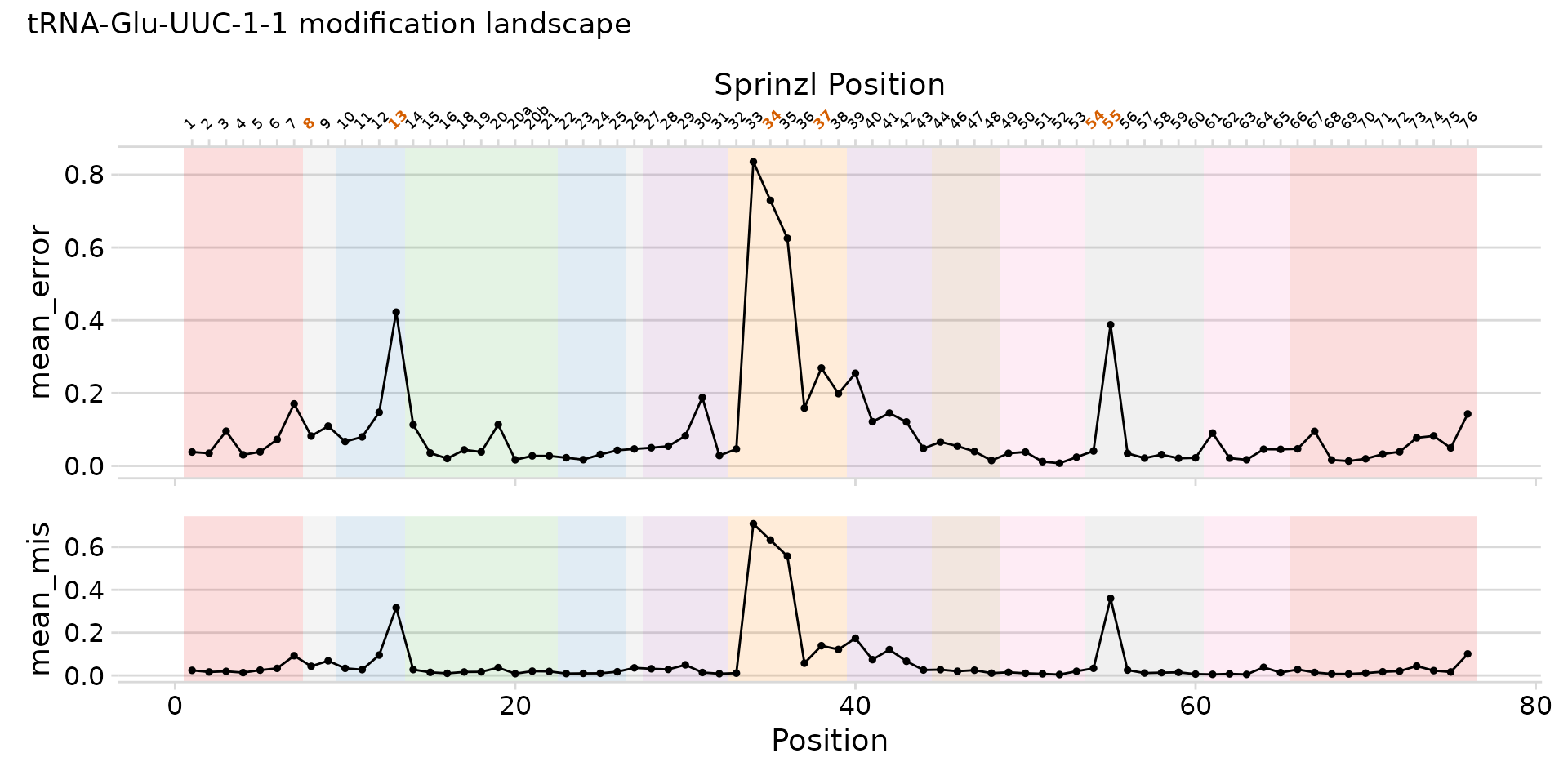
Full landscape with regions, Sprinzl axis, and modification highlights.
Heatmaps from modkit data
The heatmap workflow also supports modification data from Oxford
Nanopore’s modkit
tool. Two input formats are supported: per-read calls from
modkit extract and per-position summaries from
modkit pileup.
From modkit extract (per-read calls)
summarize_mod_calls() reads a
mod_calls.tsv.gz file (from
modkit extract --call-code) and computes per-position
modification frequency — the proportion of reads carrying a
non-canonical base call at each position.
# Summarize per-position modification frequency from each sample
wt_mods <- summarize_mod_calls("wt_sample.mod_calls.tsv.gz")
mut_mods <- summarize_mod_calls("mut_sample.mod_calls.tsv.gz")

# Bind with condition labels
mod_summary <- bind_rows(
  mutate(wt_mods, condition = "wt"),
  mutate(mut_mods, condition = "mut")
)

# Compute delta (reuses compute_bcerror_delta with mod_freq as value)
mod_delta <- compute_bcerror_delta(
  mod_summary,
  delta = wt - mut,
  value_col = "mod_freq"
)

# Prepare and plot (same workflow as bcerror data)
mod_heatmap <- prep_mod_heatmap(
  mod_delta,
  value_col = "delta",
  sprinzl_coords = sprinzl,
  mods = mods
)

plot_mod_heatmap(
  mod_heatmap,
  value_col = "delta",
  ref_col = "trna_label",
  color_limits = c(-0.5, 0.5),
  fill_name = "\u0394 mod frequency"
)
From modkit pileup (bedMethyl)
read_bedmethyl() reads the 18-column bedMethyl format
produced by modkit pileup. The percent_mod
column contains the percentage of reads with a given modification at
each position, which can be compared across conditions.
# Read bedMethyl files
wt_bed <- read_bedmethyl("wt_sample.bed.gz", min_cov = 10)
mut_bed <- read_bedmethyl("mut_sample.bed.gz", min_cov = 10)

# Bind with condition labels
bed_summary <- bind_rows(
  mutate(wt_bed, condition = "wt"),
  mutate(mut_bed, condition = "mut")
)

# Compute delta using percent_mod (0-100 scale)
bed_delta <- compute_bcerror_delta(
  bed_summary,
  delta = wt - mut,
  value_col = "percent_mod"
)

# Prepare and plot
bed_heatmap <- prep_mod_heatmap(
  bed_delta,
  value_col = "delta",
  sprinzl_coords = sprinzl
)

plot_mod_heatmap(
  bed_heatmap,
  value_col = "delta",
  ref_col = "trna_label",
  color_limits = c(-50, 50),
  fill_name = "\u0394 % modified"
)
Session info
sessionInfo()
#> R version 4.5.3 (2026-03-11)
#> Platform: x86_64-pc-linux-gnu
#> Running under: Ubuntu 24.04.3 LTS
#>
#> Matrix products: default
#> BLAS:   /usr/lib/x86_64-linux-gnu/openblas-pthread/libblas.so.3
#> LAPACK: /usr/lib/x86_64-linux-gnu/openblas-pthread/libopenblasp-r0.3.26.so;  LAPACK version 3.12.0
#>
#> locale:
#>  [1] LC_CTYPE=C.UTF-8       LC_NUMERIC=C           LC_TIME=C.UTF-8
#>  [4] LC_COLLATE=C.UTF-8     LC_MONETARY=C.UTF-8    LC_MESSAGES=C.UTF-8
#>  [7] LC_PAPER=C.UTF-8       LC_NAME=C              LC_ADDRESS=C
#> [10] LC_TELEPHONE=C         LC_MEASUREMENT=C.UTF-8 LC_IDENTIFICATION=C
#>
#> time zone: UTC
#> tzcode source: system (glibc)
#>
#> attached base packages:
#> [1] stats     graphics  grDevices utils     datasets  methods   base
#>
#> other attached packages:
#> [1] dplyr_1.2.0       clover_0.0.0.9000
#>
#> loaded via a namespace (and not attached):
#>  [1] SummarizedExperiment_1.40.0 gtable_0.3.6
#>  [3] xfun_0.57                   bslib_0.10.0
#>  [5] ggplot2_4.0.2               htmlwidgets_1.6.4
#>  [7] Biobase_2.70.0              lattice_0.22-9
#>  [9] tzdb_0.5.0                  vctrs_0.7.2
#> [11] tools_4.5.3                 generics_0.1.4
#> [13] stats4_4.5.3                parallel_4.5.3
#> [15] tibble_3.3.1                pkgconfig_2.0.3
#> [17] Matrix_1.7-4                RColorBrewer_1.1-3
#> [19] S7_0.2.1                    desc_1.4.3
#> [21] S4Vectors_0.48.0            lifecycle_1.0.5
#> [23] stringr_1.6.0               compiler_4.5.3
#> [25] farver_2.1.2                Biostrings_2.78.0
#> [27] textshaping_1.0.5           Seqinfo_1.0.0
#> [29] litedown_0.9                htmltools_0.5.9
#> [31] sass_0.4.10                 yaml_2.3.12
#> [33] pillar_1.11.1               pkgdown_2.2.0
#> [35] crayon_1.5.3                jquerylib_0.1.4
#> [37] tidyr_1.3.2                 DelayedArray_0.36.0
#> [39] cachem_1.1.0                abind_1.4-8
#> [41] commonmark_2.0.0            tidyselect_1.2.1
#> [43] digest_0.6.39               stringi_1.8.7
#> [45] purrr_1.2.1                 labeling_0.4.3
#> [47] cowplot_1.2.0               fastmap_1.2.0
#> [49] grid_4.5.3                  cli_3.6.5
#> [51] SparseArray_1.10.9          magrittr_2.0.4
#> [53] patchwork_1.3.2             S4Arrays_1.10.1
#> [55] utf8_1.2.6                  readr_2.2.0
#> [57] withr_3.0.2                 scales_1.4.0
#> [59] bit64_4.6.0-1               rmarkdown_2.30
#> [61] pwalign_1.6.0               XVector_0.50.0
#> [63] matrixStats_1.5.0           ggtext_0.1.2
#> [65] bit_4.6.0                   ragg_1.5.2
#> [67] hms_1.1.4                   evaluate_1.0.5
#> [69] knitr_1.51                  GenomicRanges_1.62.1
#> [71] IRanges_2.44.0              markdown_2.0
#> [73] rlang_1.1.7                 Rcpp_1.1.1
#> [75] gridtext_0.1.6              glue_1.8.0
#> [77] xml2_1.5.2                  BiocGenerics_0.56.0
#> [79] vroom_1.7.0                 jsonlite_2.0.0
#> [81] R6_2.6.1                    MatrixGenerics_1.22.0
#> [83] systemfonts_1.3.2           fs_2.0.1